There’s been so many times that I’ve wanted to pull location information from a website or file containing a set of addresses. This can be achieved by many hours of manual copy and pasting, a task that may even be impossible depending on the scale of the data. We can save time and sanity by making our computers do the work for us. Websites are (usually) highly organised and structured, making them perfect for programming tasks. In this post, I’ll show you how you can do this.
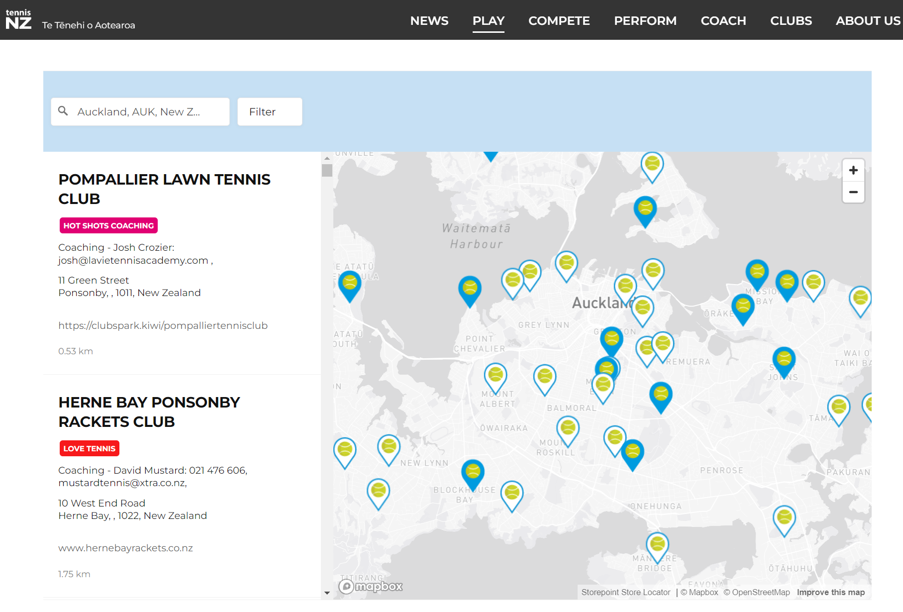
First, we want to grab data from the website we are interested in. Here’s a screen shot of Tennis NZs website showing where to play. You can see it contains a map with tennis clubs highlighted, but the information isn’t immediately accessible. You could scroll through each entry on the left (>300 clubs) and copy and paste the information out, but that’s not fun.
Map of Tennis Clubs in Auckland
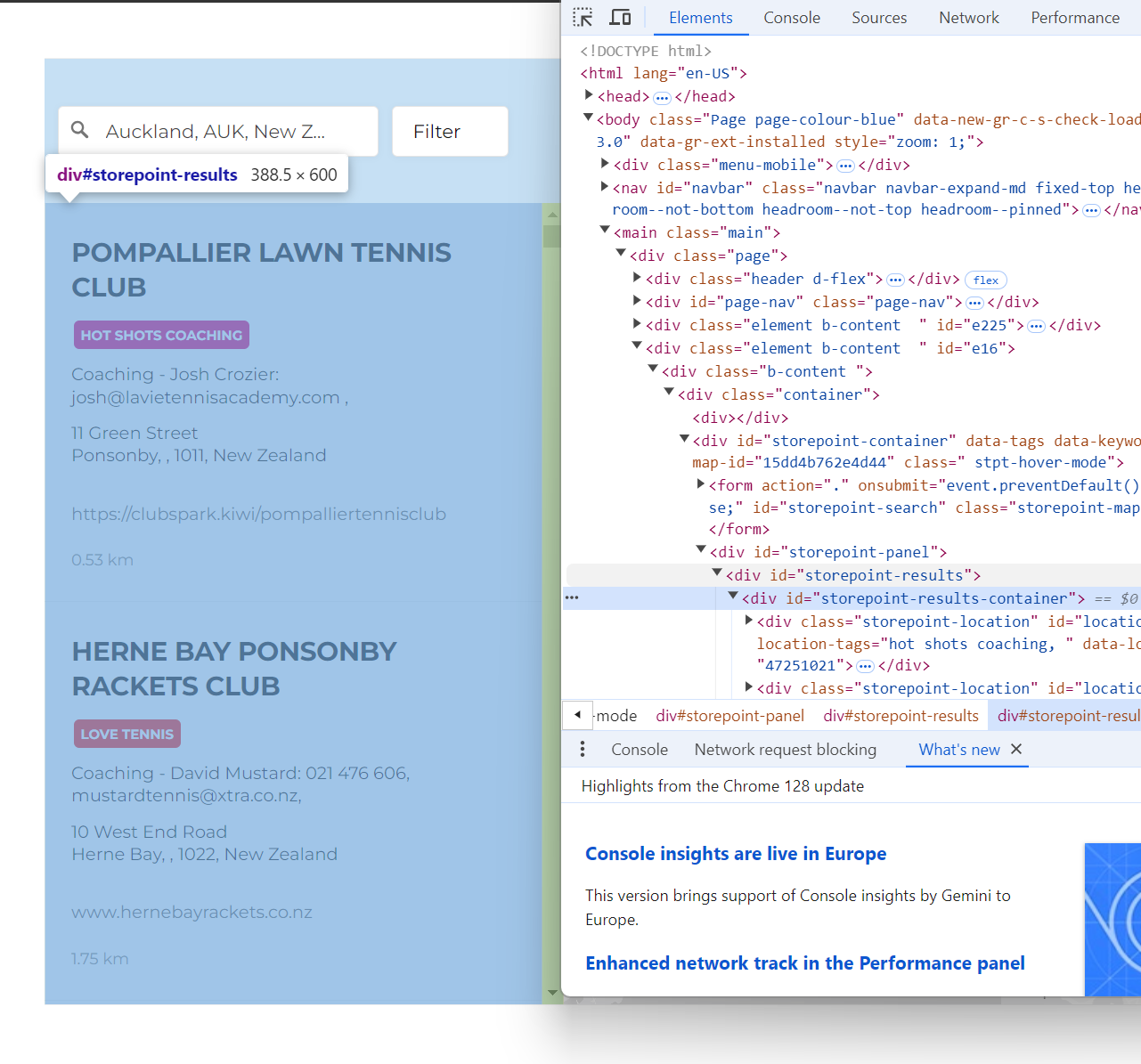
There are two ways we can pull this information. We can use the webscraper package rvest to directly pull the html from the site using read_html(website_url). For our use case ( and to ensure reproducibility), I’ll download a copy of the html directly - simply right click on the page, and click ‘save as’. We’ll have the the file Tennis NZ - Where to Play.html available for us to look at in more detail.
The code below loads this .html file. It then uses tools from the rvest package to grab the specific bits of information we are interested in. By right clicking on a webpage and clicking inspect, you can focus on the parts of the website that you are interested in. In our case, we will be pulling the contents of store-point-results
Code
library(rvest)library(dplyr)library(stringr)# Read the HTML content from the filehtml_content <-read_html(here("inputs","tennis","Tennis NZ - Where to Play.html"))# Extract addresses from elements with the class 'storepoint-address' from the HTML contentstorepoint_address_contents <- html_content |># Select elements with the class 'storepoint-address'html_elements('.storepoint-address') |># Extract text content from the selected elements and trim any surrounding whitespacehtml_text(trim =TRUE)# Also get the tags of elements with the class 'storepoint-name' from the HTML contenttag_text_contents <- html_content |># Select elements with the class 'storepoint-name'html_elements('.storepoint-name') |># Extract text content from the selected elements and trim any surrounding whitespacehtml_text(trim =TRUE)# Combine the extracted name and address data into a data frametennis_df <-data.frame(# Assign the extracted names to the 'name' columnname = tag_text_contents,# Assign the extracted addresses to the 'storepoint_address' columnstorepoint_address = storepoint_address_contents,# Prevent strings from being converted to factorsstringsAsFactors =FALSE)
As happens in 90% of cases, there are some data quality issues. For example, there’s double commas, with no content in between them. Before we can do anything with this data, we will need to fix these issues (geocoding addresses that are broken is futile!).
My code below fixes some of the issues I found in the scraped data. As an aside, regex is a game changer for cleaning data. As a Data Scientist, it’s very rare that I’ll have a day where I haven’t used some form of regex.
Code
tennis_df_clean <- tennis_df |># Add space between a lowercase letter followed by an uppercase lettermutate(storepoint_address =str_replace_all(storepoint_address, "([a-z])([A-Z])",paste0("\\1"," ","\\2" ))) |># Add space between a lowercase letter followed by a numbermutate(storepoint_address =str_replace_all(storepoint_address, "([a-z])([0-9])",paste0("\\1"," ","\\2" ))) |># Replace the abbreviation "Cnr" with "Corner"mutate(storepoint_address =str_replace_all(storepoint_address, "Cnr","Corner")) |># Remove any spaces that appear before commasmutate(storepoint_address =str_replace_all(storepoint_address, " ,","")) |># Replace any double commas with a single commamutate(storepoint_address =str_replace_all(storepoint_address, ",,",",")) |># Replace the repeated "Remuera Remuera Remuera" with a single "Remuera"mutate(storepoint_address =str_replace_all(storepoint_address, "Remuera Remuera Remuera","Remuera"))
Now we have our clean scraped data, we can focus on geocoding!
Geocode with one Simple Step
Webscraping is a simple skill opens up a world of possibilies for geospatial analysis. With the set of addresses at hand, we can add on an additional step to augment our newly pulled data with additional information. In our case, unfortutely we were unable to find any data pertaining to longitude and latidude of tennis clubs. Luckily, the tidygeocoder package makes it incredibly straight forward to get this information.
Here’s a simple chunk of code that will go through a dataset of addresses and grab the longitude and latitude.
Note, some addresses may not get a result, it depends on the quality of the addresses and the geocoding service that you use. In our case, we know the data is patchy and I’ve used open street map to geocode. Other services can be found here.
The Fruits of Our (minimal) Labour
We’ve managed to pull publically available address data, use a geocoder to get the longitude and latitude coordinates, now it time to see what we’ve got. Through a combination of ggplot2 and ggiraph, we are able to quickly visualise the newly process data points on an interactive map of Auckland. See the code below.
Code
library(sf)library(ggplot2)library(ggiraph)#load our tennis club coordinates datacoords <-read.csv(here("inputs","tennis","tennis_coords.csv")) |>filter(!is.na(latitude)|!is.na(longitude)) |>mutate(name =str_replace_all(name,"'",""))#here's a shapefile for NZ that I prepared earliernz_map <-read_sf(here("inputs","shapefiles","NZ_res01.shp"))g <-ggplot() +# Add our map of NZgeom_sf(data = nz_map,colour ="black",linewidth =0.2 ) +# Add the tennis club locations.#ggiraph makes things interactive.geom_point_interactive(data = coords,aes(x = longitude,y = latitude,tooltip = name,data_id = name ),hover_nearest = T,shape=21,size=10,colour ="white",fill ="#049030",alpha=0.7 ) +# Clip the map just to the main Auckland Areacoord_sf(xlim =c(174.5, 175.2), ylim =c(-37.1, -36.6) ) +#Styletheme_void() +theme(title =element_text(size=20)) +#Titleggtitle("Tennis Courts in Auckland, New Zealand")# wrap it in the girafe function which makes it interactivegirafe(ggobj = g,# set options for stylingoptions =list(opts_hover(css ="fill:yellow;stroke:black;stroke-width:3px;") ) )
That’s a wrap. Now that we have our data, there’s a huge number of analysis opportunities. We could look at underlying population demographics to understand access, combine it with drive times data to understand potential catchment areas,build up our visualisation to be fully customisable and interactive. At the very least, hopefully this post will save someone some time away from the computer, manually copying and pasting addresses from a website into google maps!